Line Bundling in Matplotlib

While working on a complex visualisation with points and connections in Matplotlib, I encountered quite a typical problem of unreadable output, known as a hairball in network analysis. So, what do we do about this mess? Let's try line bundling to show connections but keep them visually organised.

Line bundling is a technique used to visualize large sets of connections or edges, typically in a graph. Grouping similar lines together reduces visual clutter and helps highlight the overall structure and patterns. Line bundling has been implemented in many network libraries, including networkX in Python. But as the visualisation I am working on packs a lot, including a timeline, personal information, etc. I did not want to convert it into a networkX graph, which would make other aspects of it too complicated.

So, I decided to experiment with this by writing a couple of functions to implement line bundling directly in a Matplotlib graph, publishing the experiment here, and demonstrating how to calculate and visualize bundling points.

Visualising the problem

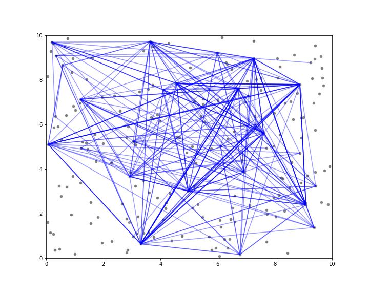
When we plot straight lines between randomly connected points, the result is often a cluttered and messy plot. As an example, I bring a case in which the connections follow a power-law distribution, which is common in many real-world networks, such as social networks. In a power-law distribution, a few nodes have many connections, while most nodes have only a few. This creates a dense web of overlapping lines that is hard to decipher.

Let's create a sample of data to visualise following the power-law distribution of connections, starting with a bunch of random points.

import numpy as np

# Sample data
np.random.seed(772)  # For reproducibility
num_points = 200
points = np.random.rand(num_points, 2) * 10

Now, lets generate a set of connections between them with a power-law distribution

import numpy as np
from scipy.stats import powerlaw

# Generate random connections using a power-law distribution
num_connections = 200
a = 0.08  # Shape parameter for the power-law distribution

# Generate a power-law distributed array and normalize it
powerlaw_distribution = powerlaw.rvs(a, size=100)
powerlaw_probabilities = powerlaw_distribution / powerlaw_distribution.sum()

# Generate indices based on the normalized power-law distribution
start_indices = np.random.choice(100, num_connections, p=powerlaw_probabilities)
end_indices = np.random.choice(100, num_connections, p=powerlaw_probabilities)

# Calculate weights based on connections
weights = np.zeros(num_points)
for start, end in zip(start_indices, end_indices):
    weights[start] += 1
    weights[end] += 1

And lets plot it out.

import matplotlib.pyplot as plt
import numpy as np

# Create a plot to visualize the points
fig, ax = plt.subplots(figsize=(10, 8))

# Scatter plot of points
ax.scatter(points[:, 0], points[:, 1], c='gray', s=20)

# Generate random connections
num_connections = 200
start_indices = np.random.choice(100, num_connections)
end_indices = np.random.choice(100, num_connections)

# Draw straight lines for each connection
for start, end in zip(start_indices, end_indices):
    ax.plot([points[start, 0], points[end, 0]], [points[start, 1], points[end, 1]], 'b-', alpha=0.2)

# Set plot limits and show the plot
ax.set_xlim(0, 10)
ax.set_ylim(0, 10)
plt.show()

As seen from this image, the powerlaw distribution, or any characteristics of this data, is not very well visible here.

Understanding Line Bundling and Bezier Curves

Line Bundling

Line bundling involves grouping lines that share similar paths. The goal is to reduce the visual complexity by merging lines into bundles. This technique is especially useful when dealing with dense graphs or networks. The intuition behind line bundling is to introduce curvature to the connections, directing them through common points or regions. As the first step, we can use Bézier curves to generate smooth curvature.

Bezier Curves

Bezier curves are parametric curves frequently used in computer graphics and related fields. They are defined by a set of control points. The most common type is the cubic Bézier curve, which is defined by four points: the start point, two control points, and the end point. Bézier curve is defined with parametric equations:

$f_x(t) := (1-t)^3 p_{1x} + 3t(1-t)^2 p_{2x} + 3t^2(1-t) p_{3x} + t^3 p_{4x}$

$f_y(t) := (1-t)^3 p_{1y} + 3t(1-t)^2 p_{2y} + 3t^2(1-t) p_{3y} + t^3 p_{4y}$

where $p_0$ and $p_3$ are the start and end points, and $p_1$ and $p_2$ are the control points. The parameter $t$ ranges from 0 to 1.

Clustering

For effective line bundling, we want to draw curves directly through common points, so "bundling" them together. For those common points, we identify central locations through which multiple lines can be routed, thereby reducing visual clutter.
We can find those central locations by clustering points, finding them as bundling points that serve as control points for the Bezier curves. Here I utilised K-Means clustering, a popular and efficient algorithm, to create these bundling points. K-Means works by partitioning the dataset into a specified number of clusters, each represented by the mean of its points, providing an effective way to identify key areas for line aggregation.

Line bundling code

First, we need to ensure that the required libraries are installed:

pip install matplotlib numpy scikit-learn scipy

Begin by importing the necessary libraries:

import matplotlib.pyplot as plt
import numpy as np
from sklearn.cluster import KMeans
from matplotlib.patches import FancyArrowPatch
from matplotlib.path import Path
from scipy.stats import powerlaw

Defining the Line Bundling Function

def add_bundled_arrow(ax, start_pos, start_y, end_pos, end_y, color, 
                      bundling_points, alpha=1, linewidth=1):
    """
    Draws a bundled arrow from start_pos to end_pos with a curvature through bundling points.
    
    Parameters:
    - ax: Matplotlib axis object.
    - start_pos: x-coordinate of the starting point.
    - start_y: y-coordinate of the starting point.
    - end_pos: x-coordinate of the ending point.
    - end_y: y-coordinate of the ending point.
    - color: Color of the arrow.
    - bundling_points: List of tuples (x, y) representing bundling points.
    - alpha: Transparency level of the lines (default 0.7).
    - linewidth: Width of the lines (default 1.5).
    """
    # Choose a bundling point closest to the midpoint of the line
    mid_x = (start_pos + end_pos) / 2
    mid_y = (start_y + end_y) / 2
    bundling_point = min(bundling_points, key=lambda bp: np.hypot(mid_x - bp[0], mid_y - bp[1]))
    
    # Create the path for the Bezier curve
    path_data = [
        (Path.MOVETO, (start_pos, start_y)),
        (Path.CURVE4, (bundling_point[0], bundling_point[1])),
        (Path.CURVE4, (bundling_point[0], bundling_point[1])),
        (Path.CURVE4, (end_pos, end_y))
    ]
    codes, verts = zip(*path_data)
    path = Path(verts, codes)
    
    # Add the path to the plot with an arrow style
    patch = FancyArrowPatch(path=path, color=color, alpha=alpha, linewidth=linewidth, arrowstyle='-|>')
    ax.add_patch(patch)

Creating Bundling Points

We will use K-Means clustering to create bundling points. Here are two functions: one for standard clustering and one for weighted clustering based on the number of connections:

def create_bundling_points(points, n_clusters=10):
    """
    Creates bundling points using K-Means clustering.
    
    Parameters:
    - points: Array of shape (n_points, 2) representing the dataset points.
    - n_clusters: Number of clusters to form (default 10).
    
    Returns:
    - bundling_points: Array of shape (n_clusters, 2) representing bundling points.
    """
    kmeans = KMeans(n_clusters=n_clusters, random_state=42).fit(points)
    bundling_points = kmeans.cluster_centers_
    return bundling_points

def create_weighted_bundling_points(points, weights, n_clusters=10):
    """
    Creates bundling points using weighted K-Means clustering.
    
    Parameters:
    - points: Array of shape (n_points, 2) representing the dataset points.
    - weights: Array of shape (n_points,) representing the weights for each point.
    - n_clusters: Number of clusters to form (default 10).
    
    Returns:
    - bundling_points: Array of shape (n_clusters, 2) representing bundling points.
    """
    # Scale points by their weights
    weighted_points = np.repeat(points, weights.astype(int), axis=0)
    
    kmeans = KMeans(n_clusters=n_clusters, random_state=42).fit(weighted_points)
    bundling_points = kmeans.cluster_centers_
    return bundling_points

Creating Bundling Points

Using the random data generated in the beginning we can use the create_weighted_bundling_points function to generate bundling points:

# Create bundling points using weighted clustering
bundling_points = create_weighted_bundling_points(points, weights, n_clusters=10)

Visualizing the Bundling Points and Connections

Finally, visualize the points, bundling points, and the bundled connections:

# Create a plot
fig, ax = plt.subplots(figsize=(10, 8))

# Scatter plot of points
ax.scatter(points[:, 0], points[:, 1], c='gray', s=20)

# Scatter plot of bundling points
ax.scatter(bundling_points[:, 0], bundling_points[:, 1], c='green', s=100, marker='x', alpha=0.4)

# Ensure no self-connections
for i in range(num_connections):
    while end_indices[i] == start_indices[i]:
        end_indices[i] = np.random.choice(100, 1, p=powerlaw_probabilities)[0]

# Draw bundled arrows for random connections
for start, end in zip(start_indices, end_indices):
    if start != end:  # Avoid self-connections
        add_bundled_arrow(ax, points[start, 0], points[start, 1], points[end, 0], points[end, 1], 
                          'red', bundling_points, alpha=0.2)

# Set plot limits and show the plot
ax.set_xlim(0, 10)
ax.set_ylim(0, 10)
plt.show()

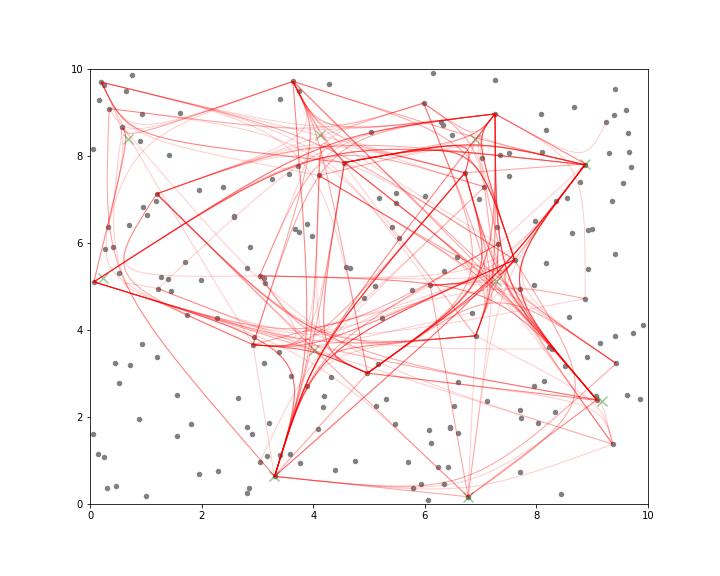
Looking at blue image in the beginning and red results here, maybe it is not the most effective way to illustrate the effects of line bundling but it certainly freed some space and it works also!

Full code

import matplotlib.pyplot as plt
import numpy as np
from sklearn.cluster import KMeans
from matplotlib.patches import FancyArrowPatch
from matplotlib.path import Path
from scipy.stats import powerlaw



def add_bundled_arrow(ax, start_pos, start_y, end_pos, end_y, color, 
                      bundling_points, alpha=1, linewidth=1):
    """
    Draws a bundled arrow from start_pos to end_pos with a curvature through bundling points.
    
    Parameters:
    - ax: Matplotlib axis object.
    - start_pos: x-coordinate of the starting point.
    - start_y: y-coordinate of the starting point.
    - end_pos: x-coordinate of the ending point.
    - end_y: y-coordinate of the ending point.
    - color: Color of the arrow.
    - bundling_points: List of tuples (x, y) representing bundling points.
    - alpha: Transparency level of the lines (default 0.7).
    - linewidth: Width of the lines (default 1.5).
    """
    # Choose a bundling point closest to the midpoint of the line
    mid_x = (start_pos + end_pos) / 2
    mid_y = (start_y + end_y) / 2
    bundling_point = min(bundling_points, key=lambda bp: np.hypot(mid_x - bp[0], mid_y - bp[1]))
    
    # Create the path for the Bezier curve
    path_data = [
        (Path.MOVETO, (start_pos, start_y)),
        (Path.CURVE4, (bundling_point[0], bundling_point[1])),
        (Path.CURVE4, (bundling_point[0], bundling_point[1])),
        (Path.CURVE4, (end_pos, end_y))
    ]
    codes, verts = zip(*path_data)
    path = Path(verts, codes)
    
    # Add the path to the plot with an arrow style
    patch = FancyArrowPatch(path=path, color=color, alpha=alpha, linewidth=linewidth, arrowstyle='-|>')
    ax.add_patch(patch)

def create_bundling_points(points, n_clusters=10):
    """
    Creates bundling points using K-Means clustering.
    
    Parameters:
    - points: Array of shape (n_points, 2) representing the dataset points.
    - n_clusters: Number of clusters to form (default 10).
    
    Returns:
    - bundling_points: Array of shape (n_clusters, 2) representing bundling points.
    """
    kmeans = KMeans(n_clusters=n_clusters, random_state=42).fit(points)
    bundling_points = kmeans.cluster_centers_
    return bundling_points

def create_weighted_bundling_points(points, weights, n_clusters=10):
    """
    Creates bundling points using weighted K-Means clustering.
    
    Parameters:
    - points: Array of shape (n_points, 2) representing the dataset points.
    - weights: Array of shape (n_points,) representing the weights for each point.
    - n_clusters: Number of clusters to form (default 10).
    
    Returns:
    - bundling_points: Array of shape (n_clusters, 2) representing bundling points.
    """
    # Scale points by their weights
    weighted_points = np.repeat(points, weights.astype(int), axis=0)
    
    kmeans = KMeans(n_clusters=n_clusters, random_state=42).fit(weighted_points)
    bundling_points = kmeans.cluster_centers_
    return bundling_points
    

# Sample data
np.random.seed(772)  # For reproducibility
num_points = 200
points = np.random.rand(num_points, 2) * 10

# Generate random connections using a power-law distribution
num_connections = 200
a = 0.08  # Shape parameter for the power-law distribution

# Generate a power-law distributed array and normalize it
powerlaw_distribution = powerlaw.rvs(a, size=100)
powerlaw_probabilities = powerlaw_distribution / powerlaw_distribution.sum()

# Generate indices based on the normalized power-law distribution
start_indices = np.random.choice(100, num_connections, p=powerlaw_probabilities)
end_indices = np.random.choice(100, num_connections, p=powerlaw_probabilities)

# Calculate weights based on connections
weights = np.zeros(num_points)
for start, end in zip(start_indices, end_indices):
    weights[start] += 1
    weights[end] += 1
    
# Create a plot to visualize the points just by straight lines
fig, ax = plt.subplots(figsize=(10, 8))

# Scatter plot of points
ax.scatter(points[:, 0], points[:, 1], c='gray', s=20)

# Generate random connections
num_connections = 200
start_indices = np.random.choice(100, num_connections)
end_indices = np.random.choice(100, num_connections)

# Draw straight lines for each connection
for start, end in zip(start_indices, end_indices):
    ax.plot([points[start, 0], points[end, 0]], [points[start, 1], points[end, 1]], 'b-', alpha=0.2)

# Set plot limits and show the plot
ax.set_xlim(0, 10)
ax.set_ylim(0, 10)
plt.show()


# Create bundling points using weighted clustering
bundling_points = create_weighted_bundling_points(points, weights, n_clusters=10)

# Create a plot
fig, ax = plt.subplots(figsize=(10, 8))

# Scatter plot of points
ax.scatter(points[:, 0], points[:, 1], c='gray', s=20)

# Scatter plot of bundling points
ax.scatter(bundling_points[:, 0], bundling_points[:, 1], c='green', s=100, marker='x', alpha=0.4)

# Ensure no self-connections
for i in range(num_connections):
    while end_indices[i] == start_indices[i]:
        end_indices[i] = np.random.choice(100, 1, p=powerlaw_probabilities)[0]

# Draw bundled arrows for random connections
for start, end in zip(start_indices, end_indices):
    if start != end:  # Avoid self-connections
        add_bundled_arrow(ax, points[start, 0], points[start, 1], points[end, 0], points[end, 1], 
                          'red', bundling_points, alpha=0.2)

# Set plot limits and show the plot
ax.set_xlim(0, 10)
ax.set_ylim(0, 10)
plt.show()